Industrial Databases: Handling Production Events at Scale
Factory data modeling in PostgreSQL, table partitioning, BRIN indexes, data retention, time series, and historians, with SQL for downtime, throughput, and OEE.

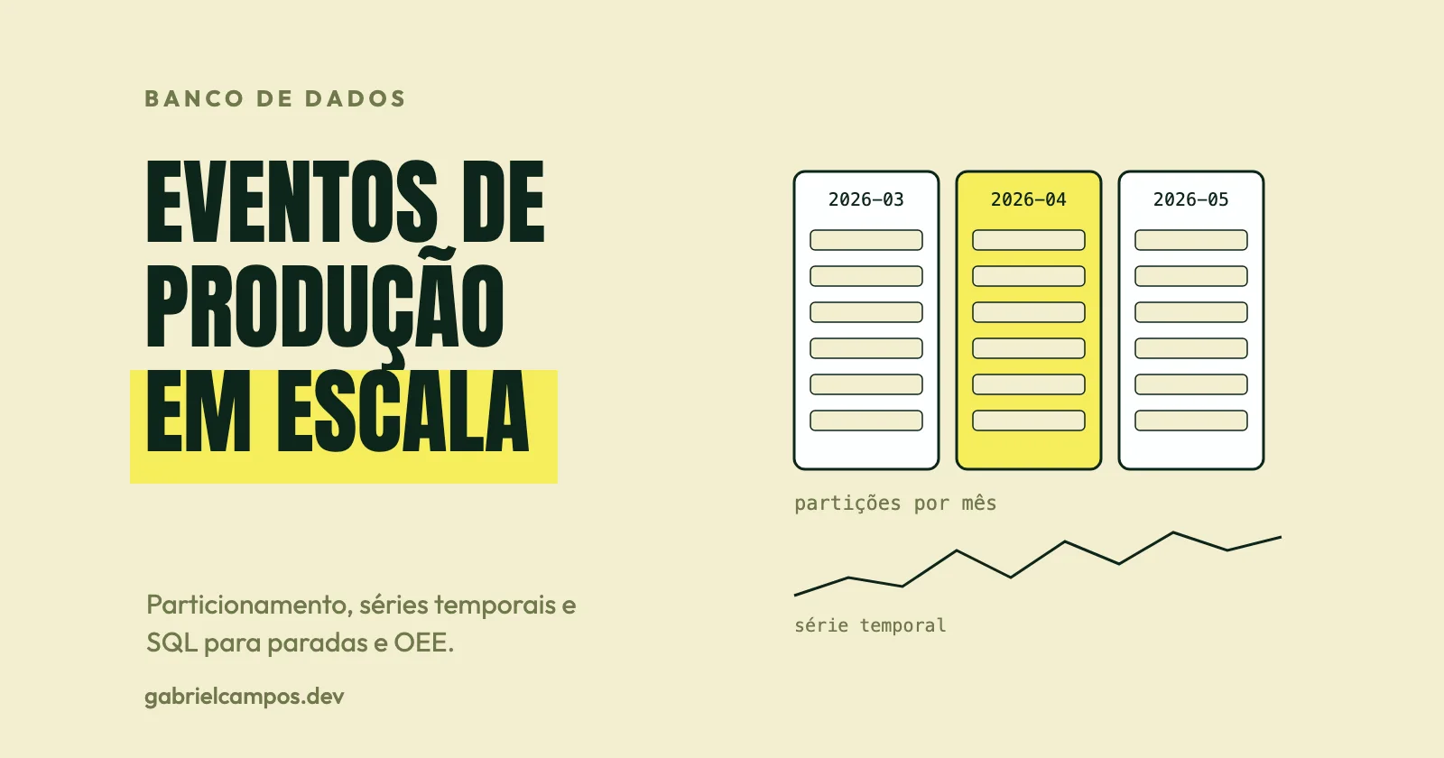
A single industrial packaging machine reporting operational state once per second produces 86,400 rows per day. Ten machines, each sampling twenty analog process variables per second, produce more than 17 million telemetry points daily. These numbers are simple arithmetic, not synthetic benchmarks, and they illustrate why manufacturing telemetry demands explicit data engineering decisions rarely encountered in standard web CRUD systems.
This is the eighth article in the series. Having explored who produces and consumes industrial data and the protocols that transport it, we examine how to persist, model, and query it.
The taxonomy of industrial factory data
Dumping all manufacturing metrics into a single catch-all table is the most common anti-pattern. There are at least five fundamentally distinct categories of factory data, each requiring different storage architectures:
- Master data: machines, lines, product SKUs, routing recipes. Low volume, slow mutation rate, demanding strict referential integrity.
- Transactional production data: work orders, lots, shift production reports, material genealogy. Moderate volume, ACID transaction boundaries, immutable auditability.
- Machine discrete events: state transitions (Running, Idle, Stopped), fault alarms, operator interventions. Medium to high volume, strictly chronologically ordered.
- Process telemetry / time series: continuous high-frequency analog sensor streams (temperature, pressure, vibration). Massive volume, append-only ingestion, queried via time-interval windows.
- Derived analytical data: pre-aggregated summaries by hour, shift, day, or facility, driving operational dashboards and OEE reporting.
This taxonomy provides a mental model (opinion) rather than a rigid normative taxonomy. Each class points toward a different database engine and indexing strategy.
Where each database technology fits
Relational databases (PostgreSQL, SQL Server, Oracle). The natural home for master data, work orders, lot traceability, and batch genealogy: ACID guarantees, foreign keys, and complex ad-hoc SQL joins. PostgreSQL comfortably ingests discrete machine events and telemetry up to substantial scales when equipped with native declarative partitioning and appropriate index strategies.
Industrial data historians. Specialized commercial platforms engineered for process tags, featuring lossy swinging-door compression, deadband filtering, temporal interpolation, and rich suites of PLC/SCADA drivers. As discussed in article 05, platforms like AVEVA PI apply exception reporting at ingress interfaces and swinging door compression in archive storage, meaning downstream queries retrieve an interpolated reconstruction of the physical signal. They represent proprietary ecosystems with proprietary query clients.
Time-series database engines.
- TimescaleDB is an extension built directly on PostgreSQL. Per its documentation, a hypertable is a PostgreSQL table automatically partitioned across time (and optionally secondary space dimensions), subdivided into chunks covering configurable time ranges; queries dynamically prune unneeded chunks. It preserves standard SQL and the PostgreSQL toolchain. Creation syntax and enterprise capabilities (lossless/lossy compression, continuous aggregates, retention policies) evolve across versions and involve edition-specific licensing; consult official documentation for your targeted release, as details are not exhaustively cataloged here.
- InfluxDB adopts a specialized time-series paradigm. In InfluxDB 3 documentation, historical measurements map to tables, tags hold indexed categorical metadata (such as
sensor_id), and fields store unindexed physical measurements; tag column definitions become immutable once established. It also supports InfluxQL, originating in v1. Architectural differences across versions (v1, v2, v3 Core/Enterprise) are substantial; verify features in vendor release notes.
Data lake / lakehouse architectures. Parquet columnar files stored on distributed object storage, queried via analytical compute engines (e.g., Trino, DuckDB, Spark). Ideal for multi-year historical archives, cross-facility benchmarking, and AI model training; far less suited for real-time shop floor dispatching. In my view, the lakehouse is a destination for derived or cold-archived factory data, never the transactional ingestion landing zone for active production lines.
No single database solves every industrial requirement. The pragmatic questions are: What is the write throughput? What is the retention horizon? What query patterns are executed? And what downtime tolerance applies?
Modeling a factory in PostgreSQL
A minimal relational schema modeling lines, machines, product SKUs, work orders, lots, machine state events, and production counts. All SQL in this article was executed and validated on PostgreSQL 17 prior to publishing.
CREATE TABLE line    (id int PRIMARY KEY GENERATED ALWAYS AS IDENTITY, code text UNIQUE NOT NULL);
CREATE TABLE machine (id int PRIMARY KEY GENERATED ALWAYS AS IDENTITY,
                      line_id int NOT NULL REFERENCES line, code text UNIQUE NOT NULL,
                      ideal_cycle_s numeric NOT NULL CHECK (ideal_cycle_s > 0));
CREATE TABLE product (id int PRIMARY KEY GENERATED ALWAYS AS IDENTITY, sku text UNIQUE NOT NULL);
CREATE TABLE work_order (id bigint PRIMARY KEY GENERATED ALWAYS AS IDENTITY, erp_no text UNIQUE NOT NULL,
                         product_id int NOT NULL REFERENCES product, qty_planned int NOT NULL);
CREATE TABLE lot (id bigint PRIMARY KEY GENERATED ALWAYS AS IDENTITY, code text UNIQUE NOT NULL,
                  work_order_id bigint NOT NULL REFERENCES work_order);

-- machine state events, partitioned monthly
CREATE TABLE machine_event (
  machine_id int NOT NULL REFERENCES machine,
  ts         timestamptz NOT NULL,
  state      text NOT NULL CHECK (state IN ('RUNNING','STOPPED','FAULT')),
  reason     text,
  PRIMARY KEY (machine_id, ts)           -- includes partition key
) PARTITION BY RANGE (ts);
CREATE TABLE machine_event_2026_03 PARTITION OF machine_event
  FOR VALUES FROM ('2026-03-01') TO ('2026-04-01');

-- production counts, with BRIN on timestamp
CREATE TABLE production_count (
  machine_id int NOT NULL REFERENCES machine, lot_id bigint NOT NULL REFERENCES lot,
  ts timestamptz NOT NULL, qty_good int NOT NULL, qty_scrap int NOT NULL DEFAULT 0,
  PRIMARY KEY (machine_id, ts)
) PARTITION BY RANGE (ts);
CREATE TABLE production_count_2026_03 PARTITION OF production_count
  FOR VALUES FROM ('2026-03-01') TO ('2026-04-01');
CREATE INDEX ON production_count USING brin (ts);
Key engineering decisions embedded in this schema:
- Composite natural key
(machine_id, ts)as primary key: prevents duplicate rows when edge buffers flush retransmissions over flaky industrial networks (idempotency, discussed in articles 06 and 07). WithINSERT ... ON CONFLICT DO NOTHING, duplicates are safely discarded without application errors. - The primary key must include the partition key column. This is an architectural constraint of PostgreSQL declarative partitioning: unique constraints on partitioned tables must encompass all columns making up the partition key.
- Recording discrete state transitions rather than continuous polling. We persist explicit transition timestamps (e.g., “transitioned to STOPPED at 10:00:00”) and derive durations dynamically. This reduces storage footprints by orders of magnitude compared to polling machine state every second, without sacrificing historical precision.
- Count granularity. In this illustrative schema, counts are logged hourly. In a live factory, ingestion granularity (per machine cycle, per minute, per pallet) represents an architectural decision directly impacting storage volume and analytical fidelity.
- Separating machine state transitions from production count tables, rather than using a polymorphic “measurements” table, ensuring data types, foreign keys, and indexes map cleanly to domain semantics.
Declarative table partitioning
PostgreSQL documentation defines three declarative partitioning methods: range, list, and hash. For temporal telemetry, range partitioning by timestamp is standard. Primary benefits:
- Partition pruning: queries containing timestamp bounds skip scanning child tables that cannot contain matching rows.
- Zero-cost retention drops: purging an aged month via
DROP TABLEorALTER TABLE ... DETACH PARTITIONavoids massiveDELETEstatements and their correspondingVACUUMtransaction bloat. - Tiered storage migration: older partition tables can be moved to cheaper storage tablespaces.
A caveat from official documentation: excessive partition counts increase query planning time and backend memory usage; too few partitions leave B-trees oversized and degrade cache locality. Benchmark with representative simulated workloads rather than guessing.
Index design: BRIN versus B-tree
For time-series telemetry inserted in strictly ascending chronological order, BRIN (Block Range Index) is an attractive choice: it stores minimum and maximum values for physical page ranges, occupying a tiny fraction of the disk footprint of a B-tree. However, BRIN is only effective when physical heap page order strongly correlates with the indexed column (e.g., an insertion timestamp). It cannot enforce uniqueness or support instant point-lookups (which require B-trees). If out-of-order data backfills disrupt correlation, BRIN efficiency degrades. The pages_per_range parameter (default 128) tunes the trade-off between index size and scan selectivity.
Automated data retention
ALTER TABLE machine_event DETACH PARTITION machine_event_2026_03;
DROP TABLE machine_event_2026_03;
With monthly range partitions, enforcing a “retain 24 months of raw events, aggregate the rest” lifecycle policy becomes a clean automated cron job: provision next month’s partition and detach or archive the oldest. A critical operational reality: in regulated industries (pharma, automotive, aerospace), traceability data retention periods are mandated by statutory regulations and customer contracts, not technical disk convenience. Discrete machine state tables and material lot genealogy tables often follow radically different retention lifecycles.
Analytical SQL: downtime analysis, availability, and OEE
Synthetic sample data models an 8-hour shift: machine 1 runs from 08:00 to 10:00, halts due to missing labels until 10:20, resumes running until 13:00, trips on a fault until 13:30, and runs until shift end at 16:00.
Identifying stoppages and calculating downtime durations
SELECT machine_id, state, reason, ts AS start_time, next_ts - ts AS duration
FROM (SELECT machine_id, ts, state, reason,
             lead(ts) OVER (PARTITION BY machine_id ORDER BY ts) AS next_ts
      FROM machine_event
      WHERE ts >= '2026-03-02' AND ts < '2026-03-03') ev
WHERE state <> 'RUNNING' AND next_ts IS NOT NULL
ORDER BY ts;
Query execution output:
 machine_id |  state  |      reason      |       start_time       | duration
------------+---------+------------------+------------------------+----------
          1 | STOPPED | missing labels   | 2026-03-02 10:00:00+00 | 00:20:00
          1 | FAULT   | level sensor err | 2026-03-02 13:00:00+00 | 00:30:00
The lead() window function pairs each transition event with its immediate successor, transforming point-in-time state transitions into contiguous duration intervals.
Shift availability, performance, quality, and OEE
WITH shift AS (SELECT '2026-03-02 08:00+00'::timestamptz AS start_t,
                      '2026-03-02 16:00+00'::timestamptz AS end_t),
ev AS (
  SELECT machine_id, state, ts,
         lead(ts) OVER (PARTITION BY machine_id ORDER BY ts) AS next_ts
  FROM machine_event, shift
  WHERE ts >= shift.start_t - interval '1 day'
),
run AS (
  SELECT machine_id, sum(least(next_ts, end_t) - greatest(ts, start_t)) AS run_t
  FROM ev, shift
  WHERE state = 'RUNNING' AND next_ts > start_t AND ts < end_t
  GROUP BY machine_id
),
prod AS (
  SELECT machine_id, sum(qty_good) AS good, sum(qty_scrap) AS scrap
  FROM production_count, shift
  WHERE ts >= start_t AND ts < end_t GROUP BY machine_id
)
SELECT m.code,
  round(extract(epoch FROM r.run_t) / extract(epoch FROM (end_t - start_t)), 3)          AS availability,
  round((p.good + p.scrap) * m.ideal_cycle_s / extract(epoch FROM r.run_t), 3)           AS performance,
  round(p.good::numeric / (p.good + p.scrap), 3)                                         AS quality,
  round(p.good * m.ideal_cycle_s / extract(epoch FROM (end_t - start_t)), 3)               AS oee
FROM run r JOIN prod p USING (machine_id) JOIN machine m ON m.id = r.machine_id, shift;
With an ideal machine cycle time of 30 seconds, the query yields Availability 0.896, Performance 0.945, Quality 0.966, and composite OEE 0.818—matching the manual mathematical verification (430 minutes runtime across 480 planned shift minutes; 785 good units and 28 scrap). Two common pitfalls in time-series SQL:
- Intervals straddling shift boundaries must be clipped using
least()andgreatest(). Filtering events strictly onts >= shift.start_tprior to evaluatinglead()drops the event that closes the initial interval, distorting calculated availability. - OEE is an organizational definition, not a universal SQL query. As emphasized in article 03, what constitutes planned operating time versus authorized breaks or ideal cycle time varies across facilities. Document the baseline calculation assumptions directly alongside the SQL query.
Verifying partition pruning
EXPLAIN (COSTS OFF)
SELECT * FROM production_count WHERE ts >= '2026-03-02' AND ts < '2026-03-03';
The planner output confirms that only production_count_2026_03 is scanned; other monthly partitions are pruned entirely from the plan tree.
Ingestion throughput, concurrency, and reliability
Micro-batched writes. Inserting telemetry row by row with single-statement transactions cripples database throughput. The standard architectural pattern collects telemetry events at the edge gateway or message broker and flushes micro-batches via multi-row INSERT statements or streaming COPY. A buffering latency of a few seconds is completely imperceptible for operational reporting, while urgent safety alarms follow dedicated real-time control paths.
Out-of-order and duplicate arrivals. Telemetry arrives delayed, duplicated, or out of order following plant network reconnects and gateway buffer flushes (article 07). Composite natural keys and ON CONFLICT DO NOTHING handle duplicate deliveries idempotently; ordering must rely on source device timestamps rather than database server ingestion time.
Explicit telemetry quality attributes. Always store a quality flag alongside physical readings (Good, Questionable, Faulted), ensuring downstream analytics never mistake an open-circuit sensor failure for a valid numeric zero.
Isolating analytical load. Heavy multi-month aggregation queries executed against active operational databases compete with write concurrency. Deploy dedicated read replicas, maintain pre-aggregated summary rollups (hourly, shift-based), or stream telemetry to an analytical warehouse.
ACID consistency boundaries. Data demanding strict relational integrity (work orders, lots, yield accounting) belongs in transactional tables guarded by foreign keys. High-frequency analog telemetry tolerates minor interpolation and loss. Attempting to force both data types into a single table structure introduces severe operational bottlenecks.
Disaster recovery. Establish clear RPO and RTO thresholds by data tier. Transactional business data demands strict point-in-time recovery; for raw sensor noise, retaining pre-computed downsampled rollups is often sufficient.
Relationship with software engineering
In my view, the most valuable software discipline is modeling manufacturing state transitions as explicit events and computing current state dynamically. Real-time dashboards, historical downtime analyses, and OEE metrics are simply queries evaluated over an immutable append-only event log, enabling full auditability, reprocessing, and retroactive bug fixes. The second rule is separating transactional business entities from high-frequency time series early in project design. The third is treating KPI definitions (OEE, availability, cycle times) as version-controlled, automated SQL code, rather than fragmented spreadsheet formulas.
Conclusion
Industrial database architectures are not monolithic: they represent a deliberate combination of relational tables for core business operations and genealogy, time-series engines or historians for high-frequency process telemetry, and analytical platforms for multi-year historical modeling. PostgreSQL—equipped with declarative range partitioning, idempotent natural keys, and BRIN indexes—handles a vast range of industrial workloads; when volume scales further, TimescaleDB, InfluxDB, or specialized historians provide purpose-built capabilities. The enduring principles remain constant: source-level timestamping, explicit quality indicators, automated partition lifecycles, and documented KPI definitions.
The next article explores IIoT and Industry 4.0, where telemetry moves beyond plant boundaries across edge gateways and cloud infrastructure.
References
This article is a study based on the sources below. Passages marked as opinion reflect my own reading. Sample data is synthetic, and all SQL statements were executed and verified on PostgreSQL 17.
- PostgreSQL Global Development Group. Table Partitioning, PostgreSQL 17 Documentation.
- PostgreSQL Global Development Group. BRIN Indexes, PostgreSQL 17 Documentation.
- Tiger Data (Timescale). Hypertables, TimescaleDB Documentation. Advanced features such as continuous aggregates, compression, and retention were not evaluated in depth in this research.
- InfluxData. Explore your schema with InfluxQL and InfluxDB 3 Core, SHOW, InfluxDB 3 Documentation.
- AVEVA. Exception reporting attributes and Data Archive, PI System Documentation (commercial historian reference).
- ISO. ISO 22400-2:2014, KPIs for manufacturing operations management (reference limited to catalog summary).
Need technical support for your software architecture or systems?
I build resilient custom web systems, high-throughput API integrations, and performance diagnostics. Direct collaboration with the engineer, zero intermediaries.
Related Articles
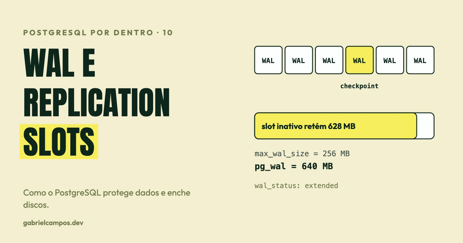
WAL, checkpoints and replication slots: how PostgreSQL protects your data (and how a forgotten slot fills the disk)
Write-Ahead Logging, full-page writes, checkpoints, crash recovery, streaming and logical replication, lag and WAL retention: how each piece works and how an abandoned replication slot becomes an incident. With experiments.
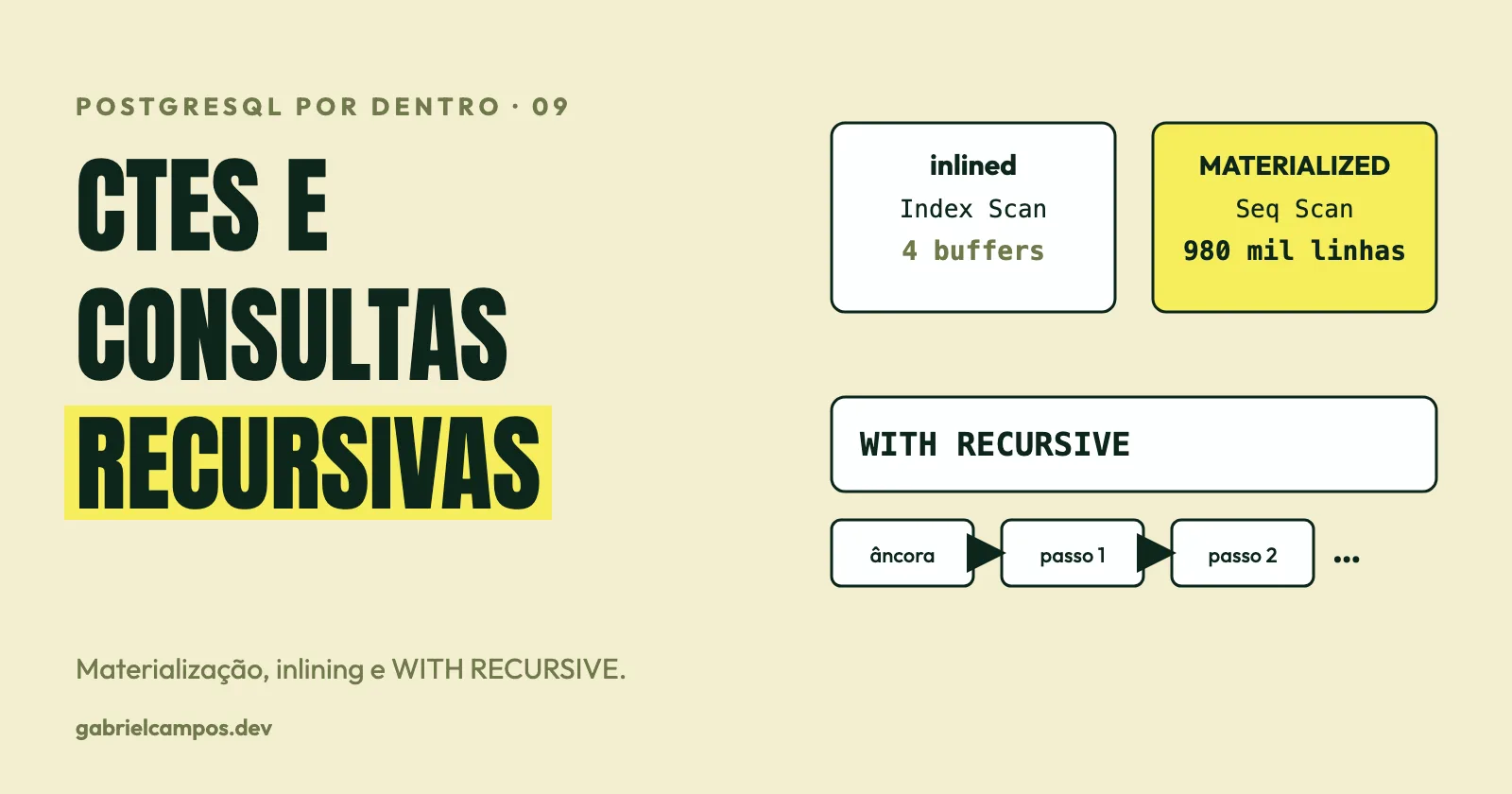
CTEs, materialization and recursive queries in PostgreSQL: what the planner does with WITH
How PostgreSQL treats CTEs since version 12: inlining, MATERIALIZED and NOT MATERIALIZED, side effects, WITH RECURSIVE, SEARCH and CYCLE, cycles in graphs and the impact on the execution plan.